2. Working with Time Series
Mauna Loa atmospheric carbon dioxide time series (1/5)
In this case study we will investigate an example of a non-linear trend which leads then to a non-linear best-fit line (non-linear means that it is not a straight line). We will also separate a data set according to a long-term trend and shorter fluctuations, caused by seasonal variabilities.
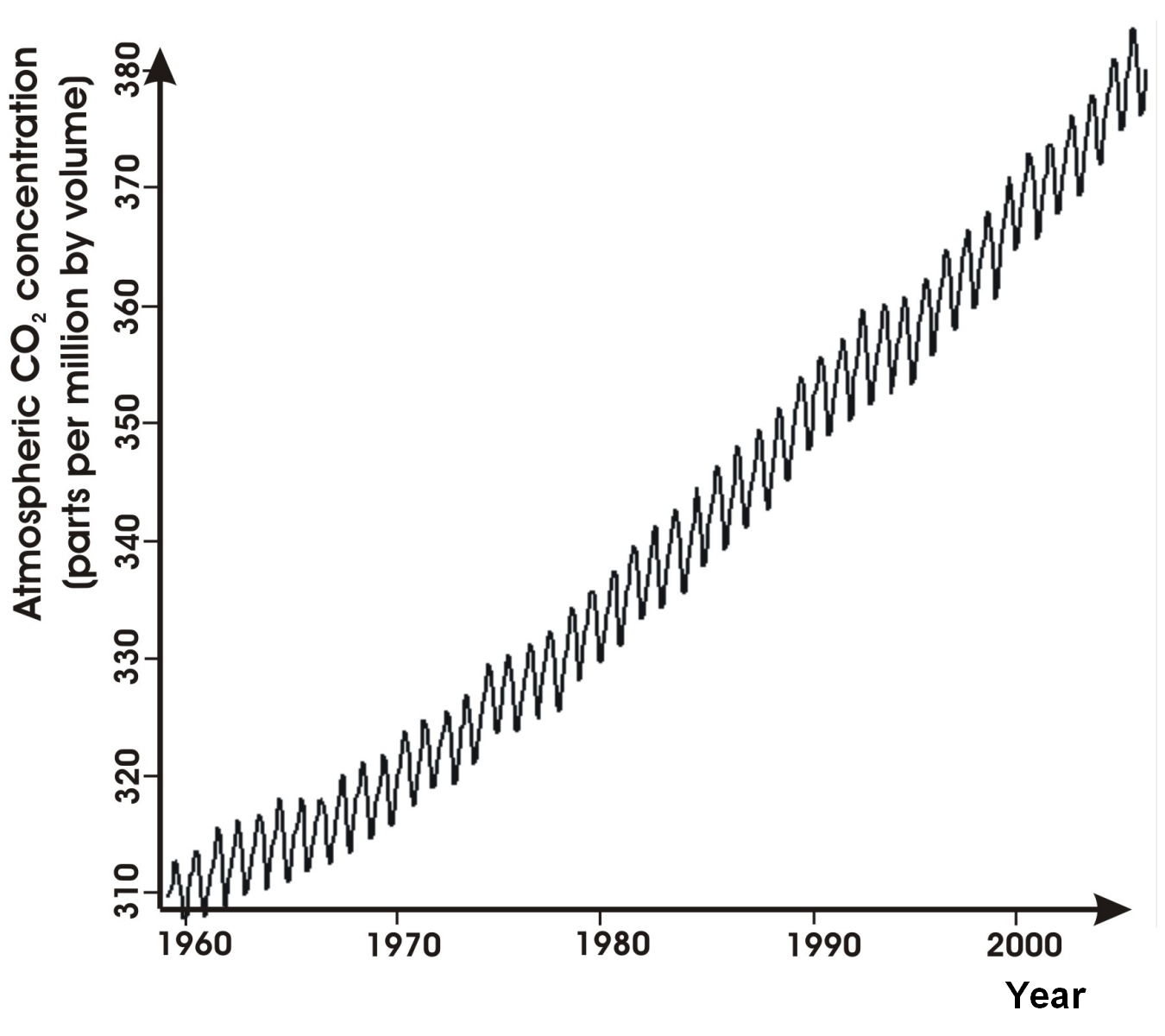
Scientists from NOAA (the US National Oceanic and Atmospheric Administration) have been measuring atmospheric carbon dioxide since 1959 near the top of the Mauna Loa volcanic cone.
The monthly values of atmospheric carbon dioxide concentration in parts per million (ppm) are shown in the graph opposite.
What does the data tell us?
You can see a regular cyclic oscillation in the data. You can see that the concentration of carbon dioxide is increasing and that the rate of increase may itself be increasing.
Splitting up the data
We can get more precise information from such a dataset by separating it into its component parts and often we can also get more information by doing so.
- The trend
- Seasonality
- The cyclic components
- The residuals
Source: NOAA Mauna Loa Laboratory
The dataset covers carbon dioxide concentrations of 313.19 to 380.63 parts per million by volume and contains 564 monthly records. We have downloaded it from http://www.esrl.noaa.gov/gmd/ccgg/trends/ for the analysis over the next few pages - you can download it too.
