2. Working with Time Series

Mauna Loa atmospheric carbon dioxide time series (2/5)

Derivation of the trend

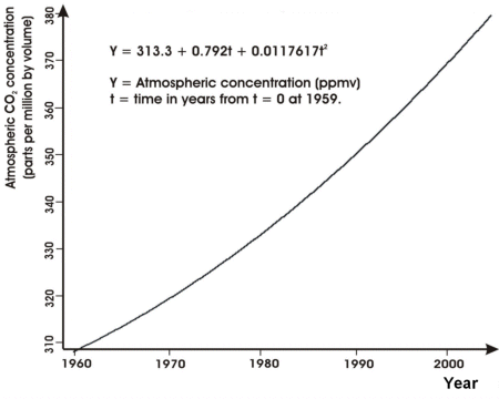
To derive the trend, we first compute annual average values for each year from the dataset. Then we fit a non-linear function to the dataset using least squares as discussed in the SEOS Tutorial Modelling of Environmental Processes. Fits using straight lines are discussed on the preceeding pages of this chapter.

In this case we will use a second order polynomial function or a parabola. The fitted function will tell us about the way that the data is changing over time.

The parabola is a good fit, with a correlation coefficient r=0.993. The parabola has the equation:

Y = 313.3 + 0.792t + 0.0117617t²

where we set t = 0 in 1959. So, from a starting value in 1959 of 313.3 parts per million, the atmospheric carbon dioxide concentration is increasing over time, and the increase is getting larger over time.

We can use this equation to estimate annual carbon dioxide levels within the period of the time series, but not necessarily beyond this period.

Questions: A closer look at the trend ↓

Why did we choose a parabola?

There are many different equations that one could choose, starting with a simple line as discussed in Tutorial 14 on Modelling of Environmental Processes. A straight line has a constant rate of change in the value of the line; but with this data the rate of change is itself changing over time.

A parabola seemed to be the simplest equation that would fit the data. But it may not give the closest fit to the data and it may not truly represent the nature of the changes that are taking place in the data.

However, without additional information, it seems to be a suitable simple model to use to analyse the actual changes that are taking place.

We can check how well the parabola fits the measurements by looking at the difference between our parabola and the actual data.

The trend in atmospheric carbon dioxide at Mauna Loa from 1959 to 2005 according to the parabolic fit to the data.

What's left?

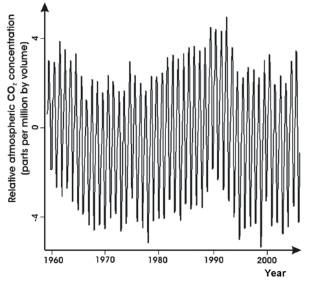
The residuals left after removing the trend are shown in the figure below.

We can see a strong cyclic component, but now we can also see something else.

There are variations over time that are not a trend, but are something else (by the way, these residuals cover the range 4.997 to -4.753 ppm).

By subtracting the trend estimated using the parabolic fit, from the actual data, we get the residuals.

What else can we get from the data?

Now we'll remove the seasonal cycle to find out.