2. Working with Time Series
Linear regression analysis (1/3)
We investigate further the methods to calculate regression lines using the Wadden Sea temperature data already discussed on the previous pages. Probably we are more interested in the July water temperatures when we spend our holidays at the seaside. The July data are shown below, as measured and monthly averaged (left graph below), and with a first guess of best-fit lines (right graph below, click on the graph titles to switch sides). Which line does best represent the data?
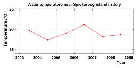
For simplicity, we change our variables from the year to x and from temperature to y. We set x=1 to January 1, 2003. July is month 7 of the year, so our first data point in the diagram is at and so on. From the Table of Wadden Sea Data we extract the water temperatures in July 2003 to 2008:
| Year | xi | yi |
| 2003 | 1.58 | 19.69 |
| 2004 | 2.58 | 17.38 |
| 2005 | 3.58 | 18.98 |
| 2006 | 4.58 | 21.12 |
| 2007 | 5.58 | 18.23 |
| 2008 | 6.58 | 18.67 |

There are several methods in geometry to define lines. We could identify two points and construct a line passing through these points; this is the two-point form of a line. In our problem it is more appropriate to find one point of the line and its slope, and so we will use the point-slope form of a line to identify the best fit regression line.
Step 1: Calculating the centroid
A point which lies on the best-fit line of our data is the centroid . The centroid can be calculated from the arithmetic mean of the xi and yi values of the data points, see supplement 1 for a detailed explanation. Let n be an integer number which denotes the number of data points. In our data set it is n=6, and it follows:

Step 2: Calculating the slope
The best-fit line shall have the smallest possible distances to the data points. How can we define these distances? The two graphs below indicate two possible procedures.
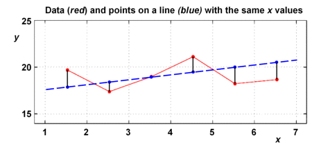
Version 2 leads to more difficult equations than version 1, and - not shown here - the calculated best-fit line would depend on the scaling of the x and y axes. One might also use a version 3, where the horizontal distances between data points and respective points on the best-fit line are used.
In our investigations we focus on version 1, i.e., the vertical distances between data points and respective points on the best-fit line. This procedure is denoted as a linear regression with respect to x.
