2. Working with Time Series
Mauna Loa atmospheric carbon dioxide time series (3/5)
Seasonality
When we look at the residuals, there is something that looks like an annual (or seasonal) cycle. This is not unexpected. Can you think of reasons why the carbon dioxide concentration varies over a year?
We can find the seasonality by computing the annual average in each year and deriving the monthly differences from this average, to give a profile for each year.
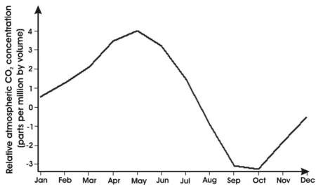
This gives us a seasonal cycle for each year, which we can then use to compute an average profile to give the seasonal component across the whole of the time series.
For this data set the maximum value in the seasonal cycle is 3.98 ppm and the minimum is -3.26 ppm.
The seasonal cycle matches the growth cycle of plants in the northern hemisphere; as plants grow they consume carbon dioxide, and so this period matches the lower levels of atmospheric carbon dioxide. In winter the reverse applies. So this is a picture of the earth breathing.
What is the problem with this cyclic component?
The problem is that we have assumed that the cyclic component does not change, and it may be changing.
To investigate this hypothesis, we calculate the time series of the seasonal cycle for the entire data set; the graph in the left column shows just the average cycle for all years in the data set. This should tell us if the cycle was different in the years around 1970 than in the years around 1990. However, growth conditions of plants are not the same in every year; this is due to e.g. a warm spring or an exceptionally cold summer, which is different from one year to the next. These annual variations should not be considered here.
One way to deal with this is to derive an average of the seasonal cycles over several years time. A single ‘good’ or ‘bad’ year in a series will then no more be an ‘outlier’ in the data set. For example, one could consider the seasonal cycle in seven years, calculate the average and associate it with the cycle of the fourth year which is the centre year in the series. The next step would be to do the same calculus with seven years that follow one year later in the time series, which yields the result for the next year; and so on... (recognising that this cannot be properly done at the start and the end of the series). This is called a moving average over the data of the time series.
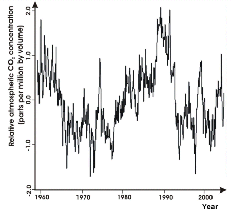
Subtracting from the time series of seasonal cycles the curve of the residuals which were obtained by subtracting the parabolic trend from the actual data (previous page, second graph in the right column) yields a result shown in the graph below.
Now look at the residuals after removing the seasonality. There is a longer term cyclic component. There may also be other, shorter term cycles but which still cross several years.
These residuals cover the range 2.077 to -1.713 ppm.


