3. Interpretation of the Linear Regression Model (2/2)

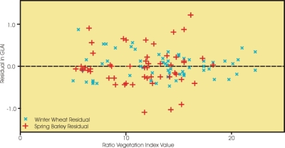
A first step in this analysis is to look at the residuals, as depicted below. Perusal of these residuals suggest that there is some pattern to the Winter Wheat residuals, with a slight dip in the residuals and then a slight rise on the right hand side. It is not very obvious, but it does suggest that a higher order polynomial might have given a slightly better fit to the data.

Residuals from fitting a linear function to the data in Table 1

The Spring Barley residuals, on the other hand, do not exhibit any significant pattern, although there are some large outliers. Although a second order polynomial does give somewhat smaller residuals for the winter wheat, let us continue to focus on the linear fitting as we move to the next lesson and consider the quality of each of the fits to the linear model.

Exercises:

1. Derive the quadratic polynomial function best fit to the data, remembering that the quadratic function is of the form b₂X²+b₁X+b₀=Y+ε so that three unknowns have to be found.


2. Repeat this process, but highlight a dataset in the graph and select Add Trendline in the local popup menu that appears when you click on a point in the dataset. Select Polynomial function of the second order and get it to display the equation and the R-squared value on the chart.