2. The Method of Least Squares (2/2)
In this equation the N represents the N observation equations since we are summing the squares of the residuals. If we place the observation equations into two arrays, then the solution of these two equations becomes relatively easy. First, place the observation equations into arrays.
where , and are the three arrays above. If we multiply both sides by the transpose of the first array, then we get
or , called the normal equations. You can easily show that the matrix equation is of the same form as the earlier equations.
From which in which is the inverse of the array.
For simple linear regression, the array is a (2, 2) array, is a (2, 1) array and is a (2,1) array, so that the normal equations can be solved directly without the need to invert the array. The two normal equations are
From which we can solve for b1 and b0
Giving
where ŷ is the estimate of y and not the actual value of y from which it differs by the residual at that observation pair.
Source: Microsoft 2003
You can import the data set of matched Ratio Vegetation Index (RVI) and Green Leaf Area Index (GLAI) data pairs for both Winter Wheat and Spring Barley into a spreadsheet and use these equations in your spreadsheet by forming the sums and the sums of products in individual cells in the spreadsheet and then solving for the two unknowns. Once you have done this for one of the crops, you can copy the cells so as to do the same for the other crop.
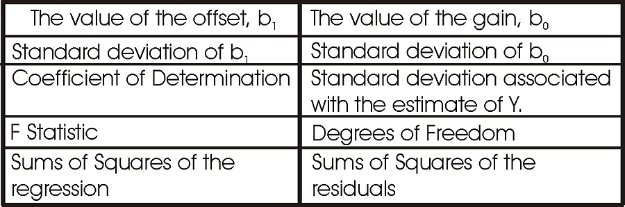
Once you have done this, try the LINEST function in Excel. To use LINEST, highlight a vacant area of two columns and five rows, and then Insert the LINEST Function into this by specifying first the Y values (GLAI), then the X values (RVI), then True and True for the remaining two input values, then simultaneously press Ctrl-Shift-Enter to have the function fill the ten locations that you have defined. Help on the LINEST function will also explain what the ten values mean. Their meaning is also given in the table above.
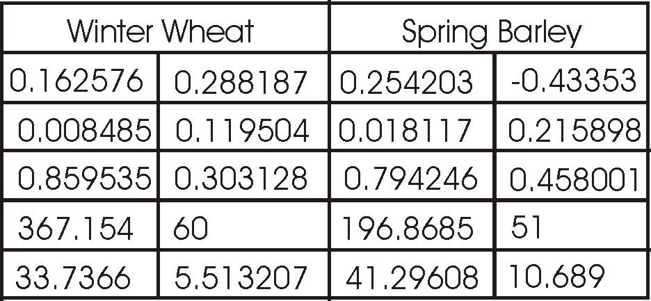
For these two datasets you should get the values as given in the table below.
Exercises
- Get the dataset referred to in the previous lesson and open it in a spreadsheet, or take the Spreadsheet created in the previous lesson. Derive the linear regression by first creating the SUMPRODUCT for the X2 and the XY terms and then summing for the X and the Y terms. Make sure that you designate the correct columns for X and Y. Then compute the two regression parameters using the appropriate equations in the notes above.
- Use the LINEST function to do the same task. You can find the two parameters values in the LINEST result, but the result contains many other things that we will meet in later lessons.
- On the graph, highlight data points in one dataset. A popup menu should appear; in this menu, choose Add Trendline, choose linear and make sure that the equation and the R2 values will appear on the plot.
- Use your derived regression equations to compute the residual values at each observation in both data sets. Create a plot of the residuals and compute the mean and variance for the residuals. What do you notice about the mean and variance?
