1. Linear Empirical Regression Models
You may have some experimental data like those shown in the figure below, taken from the data file. Access this data file and place the data into a spreadsheet, so as to produce a plot like the one shown below, but without the red and blue linear regression lines.
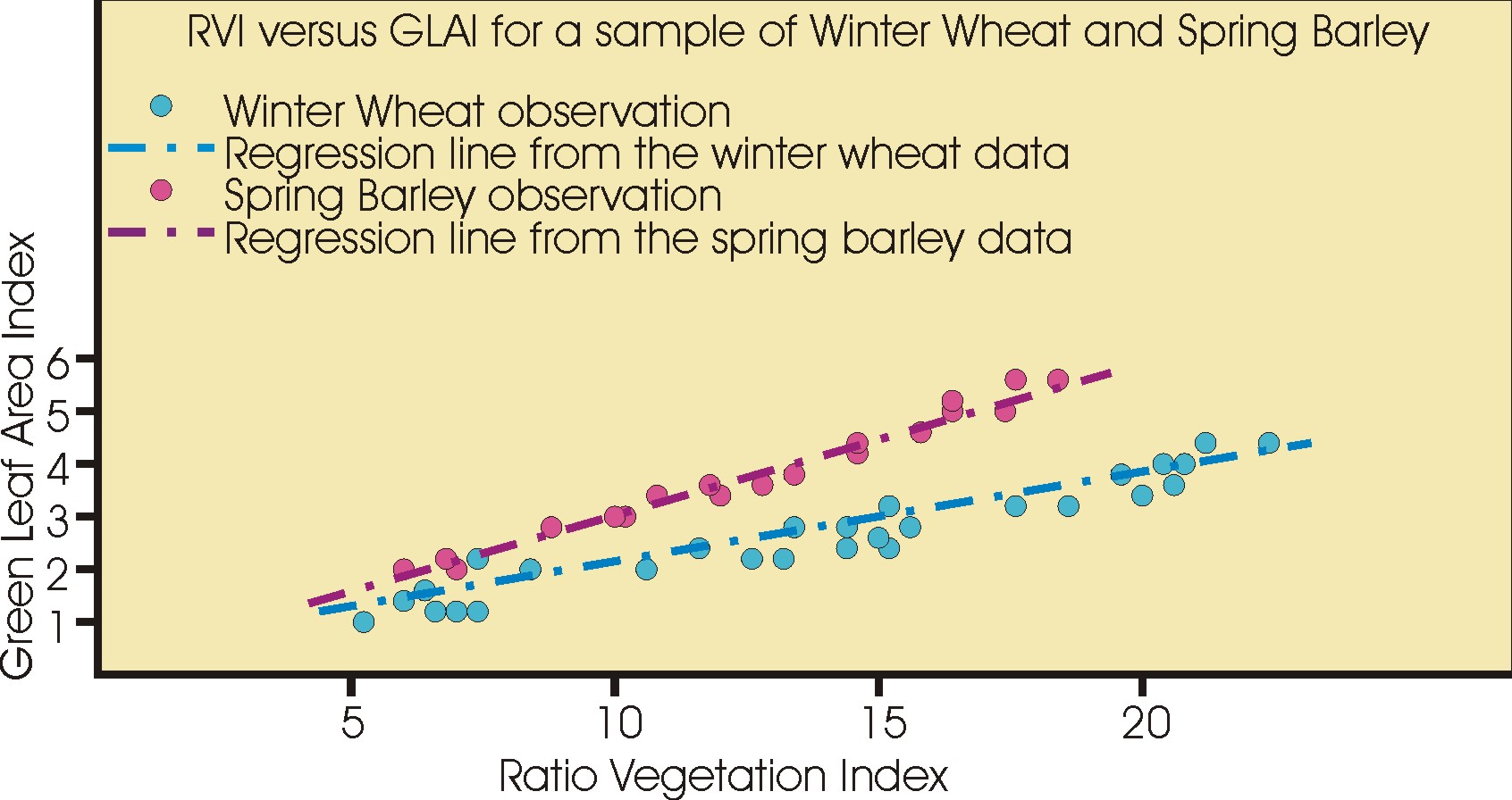
You can see that the data are highly correlated, that they do not exactly fit a line, but that a line appears to be a reasonable representation of the data. You have thus just inspected your data. Because the data are a close fit to a line, we will use a linear regression model to estimate GLAI from the Ratio Vegetation Index (RVI) data using this experimental data to build the model.
A linear model is of the form
in which b0 is also called the offset or a constant shift of the dependent variable along the y-axis (Green Leaf Area Index in this case) and b1 is called the gain or a scaling between the two variables.
In this equation there are two unknowns, the gain and the offset, so we can solve this equation if we had two values for RVI and the equivalent two values for GLAI.

But we have a lot more observations than this in the data file, 53 for the Spring Barley and 62 for the Winter Wheat. What is more, the data do not exactly fit the one line, so that for each observed value of the independent or x variable (RVI), the dependent or y variable (GLAI) is unlikely to lie exactly on the line, but be off the line by some small amount. This amount, in the y-direction, is called the residual, and it is given the symbol ε in the equation.
We have to find a way to derive the gain and offset values for a line that is a best fit to the data in accordance with some criteria. The usual criterion is that the sum of the squares of the residuals is a minimum. This is like saying that we want to find a line that fits the data with the smallest variance in the y direction. The method that we use for this is called the Least Squares Method, and it is this method that you will meet in the next lesson.
Exercises
- Access the data file and enter it into a spreadsheet, giving you four columns of data, the RVI and GLAI for both Winter Wheat and Spring Barley. Plot the data for both crop types on the same plot, but with each pair of data sets a different colour.
- Derive the mean and variance for each column of data and compute the correlation between the two parameters for both the Winter Wheat and the Spring Barley.
